

Data is everywhere and especially within Finance and Procurement. It is indispensable in tackling spend savings, contract management, supplier management, and compliance. With all of this data at their fingertips, procurement is in a prime position to use data to develop reports, perform spend analysis, evaluate suppliers and audit compliance. Data provides a framework for how teams will spend their time solving strategic business problems.
There are many ways outlier detection of spend is useful. First, it is a good way to monitor your large transactions. If a transaction is unusually high for a particular spend source, category, cost center, or account, it may be an error on your part or the vendor's. An interesting case that we've seen involves spend source. Suplari’s outlier detection’ insight flagged a P-card transaction. When the procurement team saw this, they realized the error. An employee made a purchase with a P-card rather than a purchase order. Correcting this mistake lead to more manageable spend and savings. Most importantly, knowing outliers lets you understand your organization's spend in general.
To understand outliers, we must understand some statistical concepts starting with probability distributions. I begin, as most statistics courses do, with the normal distribution.
The Normal Distribution
The normal distribution explains numerous natural phenomena. For this reason, it is a powerful tool. When examining a distribution we take note of shape, center, and spread. These descriptions determine the properties of the data and will become inputs to the outlier detector.
Shape
Shape encomposses many properties. Some words used to describe the shape of probability distributions are:
- Symmetrical or Asymmetrical
- Right or Left Skewed
- Unimodal, Bimodal, or Multimodal
- One, two, or more humps
- Thick tailed or thin tailed
- This measurement is called kurtosis
- It is relative to the normal distribution
The normal distribution is
- unimodal (one hump)
- symmetrical
- bell-shaped
Center
There are a few measures of center: mean, median, and mode. It just so happens in the case of the normal distribution, that mean, median, and mode are all equal. This is not the case with all distributions; the normal distribution has this property as a result of its shape. Mean is the measure typically used to describe probability distributions, consequently I will be referring to the center of the normal distribution as mean.
The mean is very important to know when calculating outliers. For example:
Is a transaction of $5000 an outlier?
- If the transaction is for a few laptops and the mean IT transaction is around $5000, then no.
- If it is an Uber ride and the mean transaction amount is $10, then it is probably an outlier.
The example above is obviously not a formal test of whether or not a value is an outlier. It is simply to show the intuition that the mean or center of a probability distribution will come into play during outlier detection.
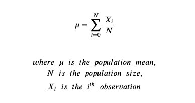
The equation for the mean is given in sigma notation below. If you are unfamiliar with sigma notation it simply states: add all the observations together and divide by the total count of observations.
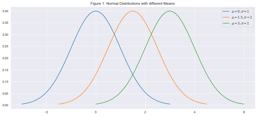
To see how different means affect the appearance the normal distribution I have plotted 3 different normal distributions with the same standard deviation, but different means in Figure 1. You can see that shifting the center shifts the entire distribution left or right. This will change the threshold for what we consider an outlier.
Spread
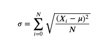
Spread refers to how the data is dispersed. Is it all bunched up near the mean, or is it very spread out? Spread can be measured with variance (?2σ2) or standard deviation (?σ). Variance is a measure of the average distance away from the mean. Since variance is often a large value, it is common practice to use standard deviation, which is simply the square root of variance. The equation for standard deviation is listed below.
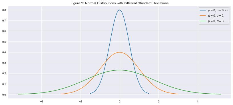
To see how different standard deviation affects the appearance of the normal distribution, I have plotted 3 different normal distributions with the same mean, but different standard deviations in Figure 2.
Outliers
An outlier is an observation that is inconsistent with the rest of the data. There are many causes of outliers. Understanding the outliers in your data helps you understand the underlying phenomena that you are studying, and improve your practices to avoid outliers caused by human errors. The Empirical Rule and IQR rule are two popular methods for identifying outliers. They are two different methods, but they essentially do the same thing. They decide on a threshold (a number). If an observation is greater than the threshold, then it is considered an outlier. What is special about calculating a statistical outlier, rather than just finding the highest value? In searching for outliers, you find what percent of your data you can expect to see in different ranges. At the end of the day, you can decide how strict you want to be about what you consider an outlier, but doing these calculations will give you a better sense and intuition for your data.
Empirical Rule
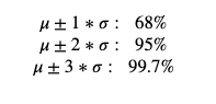
The empirical rule states that normally distributed data will have about 68% of the data contained within plus or minus 1 standard deviation from the mean. 95% of the data is contained within plus or minus 2 standard deviations from the mean and 99.7% is contained within plus or minus 3 standard deviations from the mean. The empirical rule describes how much data is contained within different sections of the distribution, but doesn't set a limit as to what constitutes an outlier. However, it is popular to consider anything beyond 3 standard deviations from the mean to be an outlier because an observation that extreme would only occur 0.3% of the time.
IQR rule
IQR stands for inter-quartile range and refers to the distance between the 75th percentile (Q3) and 25th percentile (Q1). Thus, the interquartile range finds the middle 50% of the data.
The IQR rule states that any observation that is more extreme than:
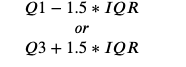
is an outlier.
The interquartile range contains 50% of the population and 1.5 * IQR contains about 99.3% of the population. If an observation lies outside of this range it means that it only occurs 0.7% of the time, which would make it rare and possibly an outlier.
Comparison
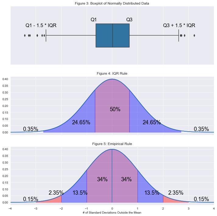
The graphic below illustrates the difference between the IQR rule and the empirical rule.
Figure 3 is a boxplot, which is another representation of the IQR rule. The line in the middle of the box is the median. The edges of the box are the 25th and 75th percentiles. The lines coming out of the boxes are sometimes called "whiskers". The dots past the ends of the whiskers are labeled as outliers according to the IQR rule.
Figure 4 is a normal distribution divided into sections according to the IQR rule. We can see that the width of the boxplot is the same as the width of the middle 50% of the distribution. The sections contained within the whiskers account for 99.3% of the data. Everything beyond the whiskers accounts for 0.7% of data.
Figure 5 is a normal distribution divided into sections according to the Empirical Rule. It describes the normal distribution in terms of standard deviations. If the threshold for outliers is set at 3 standard deviations it is slightly more restrictive than the IQR rule.
Outliers and Non-normal Distributions
What happens when we use the empirical or IQR rule on a non-normal distribution? Let's test it out! Below I generated 2000 observations from the log-normal distribution, which is right-skewed. This is a good test since most spend data is non-normal and right-skewed. The python code below generated the data.
np.random.seed(1234) # set random seed so we get same answer every time
samples=np.random.lognormal(size=2000) # sample 2000 times from lognormal distribution
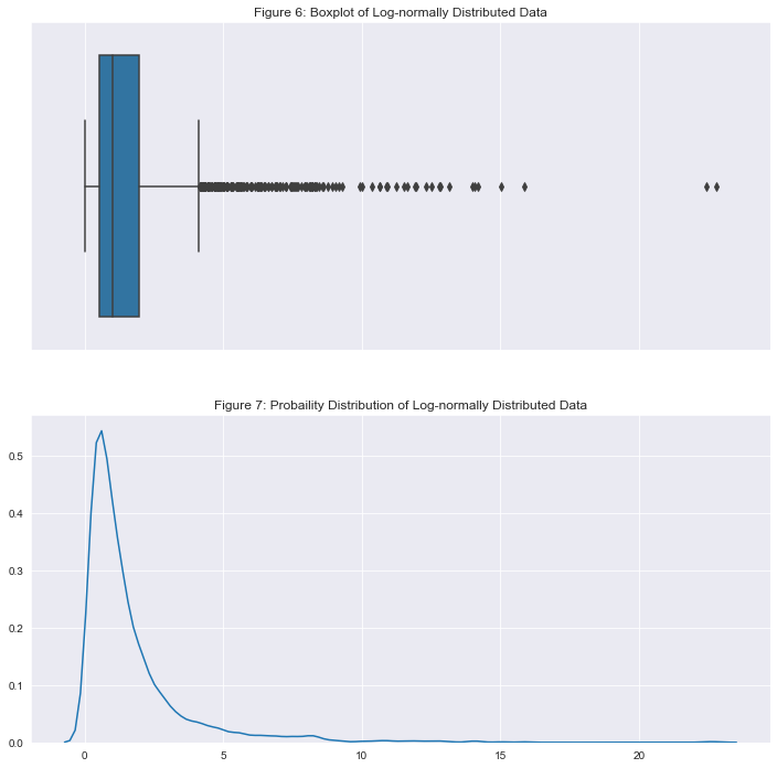
The boxplot should be throwing up red flags upon first glance. We see that the middle 50% is squeezed into the left side, there are no "outliers" on the left tail, and lots of "outliers" on the right tail.
If the IQR rule holds for this distribution, we would expect that about 0.35% of the data is beyond the right whisker in the box plot above.
To test this I find ?3+1.5∗???, which in this case is 4.11. This means that any values in the population that are greater than 4.11 are considered outliers. Next, I find the number of observations greater than 4.11 and divide by the total number of observations in the population.
I used the python code below to perform the above calculations.
threshold = np.percentile(samples, 75) + 1.5 * stats.iqr(samples) # calculate q3 + 1.5 * iqr
pct = (len(samples[samples > threshold]) / len(samples)) * 100 # find % of "outliers"
What happened!? How can 8.4% of our data be outliers? The answer is, they're not. We just happen to be working with a distribution that is skewed right. It turns out that the specifics of the IQR rule and the Empirical Rule only hold with a normal distribution. It is not useful to say that 8.4% of your data is outliers if in reality high values are common in the population of interest.
Conclusion
Today we learned a few reasons why outlier detection is useful in spend analytics. It can catch potentially fraudulent behavior, human error, and help you understand your organization's spending habits. We also learned two methods to calculate outliers when data is normally distributed: the IQR and Empirical Rules. Finally, we learned that the IQR and Empirical rules are not universal, and only work on normally distributed data.

